Yesterday the WLD club organised a workshop on spectrum analysers. I brought along my Yaesu FT-65 handheld radio and connected it, for the first time in my life, to a real spectrum analyser. What appeared on the screen was frankly fascinating, and deeply educational.
This article explains everything step by step: what the instrument is, how the test setup works, what sine waves and harmonics are, what all the units mean including the dB scale in plain language, and what CE certification has to do with it all.
Table of Contents
- What is a Spectrum Analyser, and How Does It Differ from an Oscilloscope?
- The dB Scale in Plain Language
- dBm, dB and dBc Explained with Formulas
- Sine Waves and Harmonics: the Physics of a Transmitter
- The Instrument: Siglent SSA3021X
- The Test Setup: Why 40 dB Attenuation Is Essential
- Reading the Screen: All Parameters Explained
- Marker Analysis: What Does the Screen Actually Show?
- CE Certification and What This Measurement Has to Do with It
- Summary and Conclusions
1. What Is a Spectrum Analyser, and How Does It Differ from an Oscilloscope?
The Oscilloscope: Time Domain
You may know the oscilloscope, the instrument with the green waveforms you always see in laboratory scenes. An oscilloscope shows you an electrical signal in the time domain: the horizontal axis is time, the vertical axis is amplitude (voltage).
You can literally see how the signal moves through time: the waveform. A clean radio signal at 145 MHz looks on a scope like a smooth, repeating sine wave: up, back to zero, down, back to zero, 145 million times per second.
Amplitude / Voltage (V)
    ▲
  1 |   ╭──╮       ╭──╮       ╭──╮
    |  ╯    ╰     ╯    ╰     ╯    ╰
  0 |──────────────────────────────► Time (nanoseconds)
    |        ╭─╮        ╭─╮
 -1 |         ╰──╯       ╰──╯
A scope is ideal for studying waveforms, but it does not tell you which frequency components are present, and certainly not how strong each one is individually.
The Spectrum Analyser: Frequency Domain
A spectrum analyser looks at that same signal from a completely different angle. It shows the signal in the frequency domain: the horizontal axis is frequency (in MHz), the vertical axis is power (in dBm).
Instead of “what does the signal look like over time”, a spectrum analyser asks: “which frequencies are present, and how strong is each one separately?”
Power (dBm)
    ▲
-38 |  █          ← carrier 145.96 MHz (the wanted signal)
    |  █
-93 |             █    ← 2nd harmonic (unwanted, but weak)
    |             █
-110|                       █  ← 3rd peak / spurious emission
    |─────────────────────────────► Frequency (MHz)
   120           290          434
So you can see immediately: the transmitter radiates mainly on 145.96 MHz, but there are also faint traces at higher frequencies. Those would never have been visible on an oscilloscope.
The Mathematical Bridge: Fourier
The theory behind all of this is called the Fourier transform, a mathematical technique that decomposes any arbitrary waveform into a sum of sine waves, each with their own frequency and strength. The spectrum analyser does this in hardware, in real time, while you watch.
In short: a scope shows how the signal looks. A spectrum analyser shows what it is made of.
2. The dB Scale in Plain Language
This is the section where many people switch off. “dB”, “dBm”, “dBc”: it sounds complicated, but the idea behind it is actually quite elegant. Read through this carefully, because once you understand it, the rest of the article falls into place.
The Problem with Linear Scales
Suppose you want to show on a single graph both the power of a broadcast transmitter (100,000 Watts) and the weakest signal a receiver can still detect (0.000 000 001 Watt = 1 nW).
Using a normal linear scale (1, 2, 3, 4…) the graph would look like this:
Power (W)
100,000 |                                          ████ ← transmitter
        |
        |
        |
        |
      0 |████████████████████████████████████████████── everything below ~1 W invisible here
          receiver  radio  torch  lamp    mast
The receiver and radio are literally not visible at that scale. That is the problem when dealing with enormously large numerical ranges.
The Solution: Logarithms
A logarithm is a mathematical way to make large numbers manageable. Instead of “how large is the number”, you ask: “to what power must I raise 10 to get that number?”
Some examples:
| Number | Logarithm (log₁₀) | Explanation |
|---|---|---|
| 1 | 0 | 10⁰ = 1 |
| 10 | 1 | 10¹ = 10 |
| 100 | 2 | 10² = 100 |
| 1,000 | 3 | 10³ = 1,000 |
| 1,000,000 | 6 | 10⁶ = 1,000,000 |
| 0.1 | −1 | 10⁻¹ = 0.1 |
| 0.001 | −3 | 10⁻³ = 0.001 |
The magic: every number, large or small, now fits onto a manageable scale.
From Logarithm to Decibel (dB)
The decibel is a unit based on the logarithm. “Deci” = one tenth, “Bel” = named after Alexander Graham Bell. The definition for power:
dB = 10 × log₁₀(ratio)
This sounds abstract. Let us make it concrete with an example.
The Ratio Table: dB in Plain Terms
Suppose you compare two loudspeakers. Speaker A outputs 1 Watt. Speaker B outputs 2 Watts. How large is the difference in dB?
dB = 10 × log₁₀(2/1) = 10 × 0.301 = 3 dB
3 dB difference = twice the power. That is the single most important dB rule.
Here is a table worth keeping:
| Power ratio | dB | In plain language |
|---|---|---|
| ÷ 1,000,000,000 | −90 dB | one billion times weaker |
| ÷ 1,000,000 | −60 dB | one million times weaker |
| ÷ 1,000 | −30 dB | one thousand times weaker |
| ÷ 100 | −20 dB | one hundred times weaker |
| ÷ 10 | −10 dB | ten times weaker |
| ÷ 2 | −3 dB | twice as weak |
| × 1 | 0 dB | equal strength |
| × 2 | +3 dB | twice as strong |
| × 10 | +10 dB | ten times stronger |
| × 100 | +20 dB | one hundred times stronger |
| × 1,000 | +30 dB | one thousand times stronger |
| × 1,000,000 | +60 dB | one million times stronger |
💡 Rule of thumb: every factor of 10 in power = +10 dB. Every factor of 2 = +3 dB. Negative = weaker, positive = stronger.
The Power of Addition and Subtraction in dB
Here is where things get really useful. In the ordinary world you must multiply powers when combining them (an amplifier with gain ×100 after a cable with loss ×0.5 = ×50 total). In the dB world you simply add:
Amplifier:  +20 dB
Cable:       −3 dB
─────────────────────
Result:     +17 dB  (= factor 50)
That is precisely why radio amateurs and engineers always think in dB. It makes complex signal chains immediately transparent.
The Logarithmic Scale on Screen
Now you also understand why the spectrum analyser uses a logarithmic scale. On the screen we see 8 dB per grid row (LOG 8 dB). Each row downward is 8 dB weaker, a factor of 6.3 in power. Over 10 rows from top to bottom that is a factor of 6.3¹⁰ ≈ one billion. That enormous range fits visually and neatly on the screen.
Row  1 (top):   −40 dBm  = 0.0001    mW  ← reference line
Row  2:         −48 dBm  = 0.000016  mW
Row  3:         −56 dBm  = 0.0000025 mW
...
Row 10 (bottom):−112 dBm = 0.000000000006 mW  ← noise floor
On a linear scale this would be impossible to draw. Logarithmically: just 10 rows.
3. dBm, dB and dBc Explained with Formulas
Now that we understand the dB scale, we can discuss the specific units shown on screen.
dBm: Absolute Power
dBm stands for decibels relative to 1 milliwatt, an absolute power measure: you know exactly how many Watts it represents, not just the ratio to something else.
The formula:
P(dBm) = 10 × log₁₀( P(mW) / 1 mW )
In reverse (from dBm to Watts):
P(mW) = 10 ^ ( P(dBm) / 10 )
A reference table every radio amateur should know by heart:
| Power | dBm | Typical context |
|---|---|---|
| 100 W | +50 dBm | HF station full power |
| 50 W | +47 dBm | Typical HF base station |
| 25 W | +44 dBm | Class C licence limit |
| 5 W | +37 dBm | FT-65 high power |
| 500 mW | +27 dBm | FT-65 low power |
| 100 mW | +20 dBm | QRP transmit power |
| 1 mW | 0 dBm | Reference point by definition |
| 100 µW | −10 dBm | Strong received signal |
| 1 µW | −30 dBm | Normal received signal |
| 100 nW | −40 dBm | Reference line on our screen |
| 1 nW | −60 dBm | Weak but usable signal |
| 0.001 nW | −90 dBm | Edge of usable signal |
| 0.000001 nW | −120 dBm | Typical noise floor of a sensitive receiver |
dB: Relative Difference
dB (without suffix) is always a ratio between two powers. It has no absolute meaning: it only says how large the difference is.
ΔdB = 10 × log₁₀( P1 / P2 )
On our screen we see marker ΔM1 with 73.09 dB. That means:
Ratio = 10 ^ (73.09 / 10) = 10 ^ 7.309 = 20,380,000
The carrier is therefore more than 20 million times stronger than the noise floor. That is why we need the dB scale: on a linear scale this simply cannot be displayed.
dBc: Spectral Purity
dBc stands for decibels relative to the carrier, the desired primary frequency of the transmitter.
P(dBc) = P(spur, dBm) − P(carrier, dBm)
This is the measure of how cleanly a transmitter radiates. The more negative, the better.
Example: if the carrier is −37.73 dBm and a harmonic is −93.10 dBm:
P(dBc) = −93.10 − (−37.73) = −55.37 dBc
The harmonic is therefore 55.37 dB weaker than the carrier. That is a factor of:
10 ^ (55.37 / 10) = 344,000 × weaker
4. Sine Waves and Harmonics
The Ideal Sine: What a Transmitter Tries to Produce
A transmitter tries to generate one pure sine wave on the desired frequency. Mathematically:
s(t) = A × sin(2π × f₀ × t)
where:
- A = amplitude (signal strength)
- f₀ = fundamental frequency (the desired transmit frequency, e.g. 145.96 MHz)
- t = time
On a spectrum analyser this would give one perfect, infinitely narrow line at f₀, and beyond that… absolute silence.
Reality: Harmonics Are Inevitable
In practice, a perfect sine wave does not exist. Transistors, amplifier stages, switching power supplies and other components inside a transmitter are not perfectly linear, they distort the signal slightly. That distortion has a mathematically predictable consequence: harmonics are generated.
Harmonics are additional sine waves at exact multiples of the fundamental frequency:
s(t) = A₁×sin(2π×f₀×t)        ← fundamental (wanted)
     + A₂×sin(2π×2f₀×t)       ← 2nd harmonic (unwanted)
     + A₃×sin(2π×3f₀×t)       ← 3rd harmonic (unwanted)
     + A₄×sin(2π×4f₀×t) + ...
This is not a coincidence or design flaw: it is a fundamental law of mathematics (Fourier analysis): any non-linear distortion of a sine wave produces harmonics at multiples of the fundamental frequency.
Harmonics of the FT-65 at 145.96 MHz
| Harmonic | Calculated frequency | Measured on screen | Deviation |
|---|---|---|---|
| 1st (fundamental) | 145.960 MHz | 145.960 MHz | 0 |
| 2nd harmonic | 291.920 MHz | ~291.600 MHz | ~320 kHz* |
| 3rd harmonic / spur | 437.880 MHz | ~434.160 MHz | ~3.7 MHz** |
* Small deviation due to the wide RBW of 300 kHz, acceptable at this measurement setting.
** Larger deviation: this is likely a spurious emission from the radio’s internal synthesiser, not the true third harmonic.
Why Harmonics Can Never Be Fully Eliminated
Even the most expensive professional transmitters have harmonics: they are simply suppressed to an extremely low level. The goal of good transmitter design is to push those harmonics as far below the carrier as possible, so they cause no interference to other users of the radio spectrum.
💡 Analogy: think of an acoustic guitar. When you pluck a string, you hear not just the fundamental note but also the overtones (harmonics). That is precisely what makes the string sound beautiful. In a radio transmitter, however, you want those overtones to be as small as possible, because they could interfere with other stations.
5. The Instrument: Siglent SSA3021X
What Is the Siglent SSA3021X?
The Siglent SSA3021X is a professional mid-range spectrum analyser made by the Chinese manufacturer Siglent, a respected maker of test equipment that is also found in professional laboratories.
| Specification | Value |
|---|---|
| Frequency range | 9 kHz – 2.1 GHz |
| Dynamic range | >98 dB |
| Phase noise performance | −98 dBc/Hz @ 10 kHz offset |
| Minimum RBW | 1 Hz |
| Maximum input power | +20 dBm (absolute maximum) |
| Display | 10.1” touchscreen |
| Connectivity | USB, LAN |
| Indicative price | ~€1,500 – €2,000 |
What Does the Frequency Range Cover?
With its upper limit of 2.1 GHz, the SSA3021X covers the entire playground for VHF/UHF radio amateurs:
| Amateur band | Frequency | Covered? |
|---|---|---|
| HF | 1.8 – 30 MHz | ✅ |
| 6m | 50 – 54 MHz | ✅ |
| 2m | 144 – 146 MHz | ✅ |
| 70cm | 430 – 440 MHz | ✅ |
| 23cm | 1240 – 1300 MHz | ✅ |
| 13cm | 2300 – 2450 MHz | ❌ just outside range |
For most VHF/UHF measurements this instrument is more than sufficient.
What Can You Measure with It?
A spectrum analyser like the SSA3021X is used for:
- Harmonic analysis: as in this article
- Channel power and occupancy: how much spectrum does your signal consume?
- Intermodulation: distortion when two signals are present simultaneously
- Antenna match curves: in combination with a tracking generator
- EMC pre-compliance: are there unwanted emissions from equipment?
- Spectrum monitoring: which signals are active in a given range?
6. The Test Setup: Why 40 dB Attenuation Is Essential
The Problem: Too Much Power
The Yaesu FT-65 is a handheld radio with a maximum transmit power of 5 Watts. In dBm:
P = 10 × log₁₀(5000 mW / 1 mW) = 10 × log₁₀(5000) = 10 × 3.699 = +36.99 dBm ≈ +37 dBm
The maximum safe input of the Siglent SSA3021X is +20 dBm (= 100 mW). The difference:
+37 dBm (transmitter) − +20 dBm (max analyser) = 17 dB too much
17 dB too much = well over 50 times the maximum permitted power. That would permanently and instantly destroy the sensitive FET input stage of the analyser.
⚠️ Golden rule when using a spectrum analyser:
Never connect a transmitter without first checking that the input power of the analyser is not exceeded. A damaged analyser input is an expensive mistake.
The Solution: a 40 dB Attenuator
Between the antenna output of the FT-65 and the RF INPUT of the SSA3021X, a 40 dB attenuator (signal reducer) was placed.
┌──────────┐  SMA   ┌───────────────┐  SMA  ┌──────────────────┐
│ Yaesu    │ ──────►│  40 dB        │ ─────►│ Siglent SSA3021X │
│  FT-65   │        │  Attenuator   │       │   RF INPUT       │
│  Low pwr │        │               │       │   max +20 dBm    │
└──────────┘        └───────────────┘       └──────────────────┘
  +27 dBm              − 40 dB                 −13 dBm  ✅ safe
  (500 mW)           (factor 10,000)            (50 µW)
What Is an Attenuator?
An attenuator is a precision passive network of resistors. It reduces the signal power by an exact, known factor: in this case 10,000 times (= 40 dB), without altering the frequency content or the relative ratios between signal components.
This is crucial: both the carrier and all harmonics are attenuated equally. The relative ratios (dBc) remain identical, even after the attenuator. This means we can still correctly measure harmonic suppression.
Attenuator in the Signal Chain
Signal at the FT-65 antenna output (Low Power):
    Carrier:          +27.00 dBm
    2nd harmonic:     +27.00 − 55.37 = −28.37 dBm
    3rd peak / spur:  +27.00 − 71.80 = −44.80 dBm

After 40 dB attenuator (measured values at analyser input):
    Carrier:          +27.00 − 40 = −13.00 dBm  (theoretical)
    Measured:                       −37.73 dBm   (extra cable loss + measurement uncertainty)
    2nd harmonic:                 ~ −93.10 dBm
    3rd peak / spur:              ~ −109.53 dBm
The difference between the theoretical −13 dBm and the measured −37.73 dBm (~25 dB) is due to cable losses, the internal measurement configuration, and possible deviations in the exact attenuation of the attenuator. For a qualitative harmonic analysis this does not matter: what we care about are the relative levels (dBc), not the absolute values.
7. Reading the Screen: All Parameters Explained
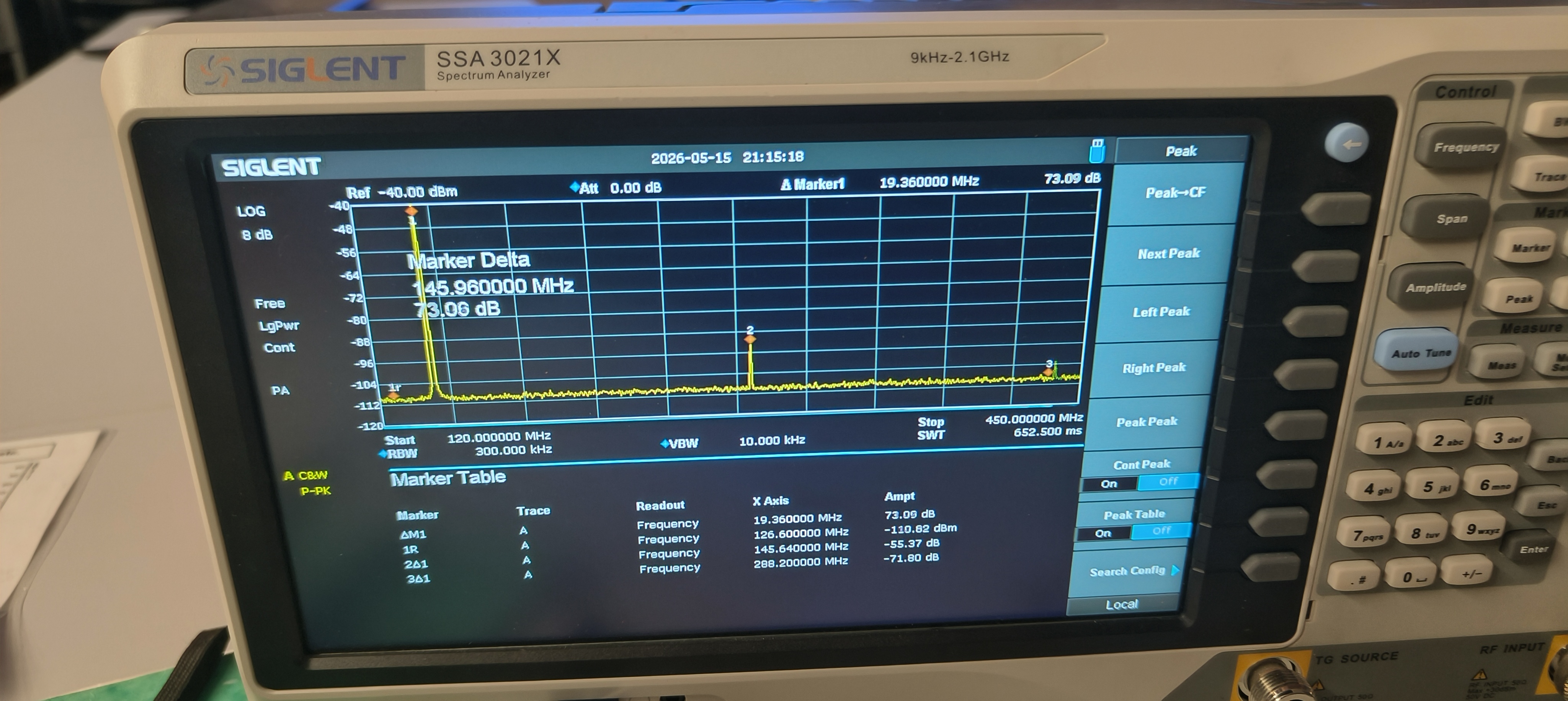
The photo below shows the Siglent SSA3021X screen as captured during the measurement on 15 May 2026.
Fundamental Settings of the Measurement
| Parameter on screen | Value | What does it mean? |
|---|---|---|
| Ref −40.00 dBm | −40 dBm | Top of the Y-axis (reference line at top) |
| LOG 8 dB | 8 dB/division | Each grid row = 8 dB difference in power |
| Att 0.00 dB | 0 dB | No additional internal attenuation in the analyser |
| RBW 300 kHz | 300 kHz | Resolution bandwidth, width of the measurement filter |
| VBW 10 kHz | 10 kHz | Video bandwidth, noise smoothing |
| Start 120 MHz | 120 MHz | Left edge of the graph |
| Stop 450 MHz | 450 MHz | Right edge of the graph |
| Span ~330 MHz | 330 MHz | Total measured frequency range |
| SWT 652.5 ms | 652.5 ms | Time for one complete sweep from left to right |
RBW and VBW: What Are They?
RBW (Resolution BandWidth) is the width of the internal measurement filter. You can think of it as the aperture of a magnifying glass sliding across the spectrum:
- Narrow RBW (e.g. 1 kHz): you see a lot of detail, but the sweep takes longer. Suitable for accurate measurement of weak signals.
- Wide RBW (e.g. 300 kHz): you quickly get an overview but lose detail. Suitable for an initial survey.
In this measurement RBW = 300 kHz was used, wide enough to capture the entire 2m FM signal (including the modulation sidebands) in one broad peak. For norm-compliant measurements you would use a narrower RBW.
VBW (Video BandWidth) is a smoothing filter that averages out noise fluctuations so that weak signals become more visible. A low VBW gives a quieter, more averaged display.
Reading the Y-Axis
The Y-axis shows LOG 8 dB per division. The scale runs (top to bottom):
−40 dBm  ← reference line (top grid)
−48 dBm
−56 dBm
−64 dBm
−72 dBm
−80 dBm
−88 dBm
−96 dBm
−104 dBm
−112 dBm  ← noise floor (~bottom grid)
The carrier peak reaches just below −40 dBm. The noise floor sits around −110 dBm. That is a dynamic range of 70 dB; in other words, the test setup distinguishes signals that differ by a factor of 10,000,000 in power.
8. Marker Analysis: What Does the Screen Actually Show?
The SSA3021X uses a delta-marker system in this measurement. Here is how it works:
- 1R = the reference marker, manually placed on the noise floor (no signal). This is the zero reference for all delta measurements.
- ΔM1 = the delta relative to 1R. This shows the difference from the reference.
- 2Δ1, 3Δ1 = additional delta-markers relative to the carrier.
Marker 1R: the Noise Floor
Frequency: 126.600 MHz
Power:     −110.82 dBm
This is the noise floor of the test setup, the lowest level we can measure. In power terms: 10^(−110.82/10) = 0.0000000083 mW = 8.3 picowatts. An unimaginably small quantity.
Marker ΔM1: the Carrier
Delta frequency: +19.360 MHz
Delta power:     +73.09 dB

Actual frequency: 126.600 + 19.360 = 145.960 MHz  ✅ (2m FM segment)
Actual power:     −110.82 + 73.09  = −37.73 dBm
The carrier sits at 145.960 MHz, a standard 2m frequency, and has a power of −37.73 dBm at the analyser input (after the 40 dB attenuator).
Marker 2Δ1: the Second Harmonic
Delta frequency relative to carrier: +145.640 MHz
Actual frequency: 145.960 + 145.640 = 291.600 MHz
Delta power: −55.37 dBc

Expected 2nd harmonic: 145.960 × 2 = 291.920 MHz
Deviation: ~320 kHz (acceptable with RBW = 300 kHz)
Power at analyser input: −37.73 + (−55.37) = −93.10 dBm
Marker 3Δ1: the Third Peak
Delta frequency relative to carrier: +288.200 MHz
Actual frequency: 145.960 + 288.200 = 434.160 MHz
Delta power: −71.80 dBc

Expected 3rd harmonic: 145.960 × 3 = 437.880 MHz
Deviation: ~3.7 MHz (too large for a true harmonic)
The deviation of nearly 4 MHz is too large to confidently call this the third harmonic. This is most likely a spurious emission, an unwanted signal component from the radio’s internal VCO or PLL synthesiser, rather than a true harmonic. Its level of −71.80 dBc is well below the regulatory limit, so no cause for concern.
9. CE Certification and What This Measurement Has to Do with It
What Is CE Certification?
CE (Conformité Européenne) is the European certification mark. When you see a CE mark on a product, it means the manufacturer declares that the product complies with all applicable European directives.
For radio transmitters, including the Yaesu FT-65, this falls under the Radio Equipment Directive (RED) 2014/53/EU. Concretely, the manufacturer must demonstrate that the device:
- Has spectral purity: harmonics and unwanted emissions are sufficiently suppressed
- Does not interfere with other equipment: EMC (electromagnetic compatibility)
- Is safe for the user: electrical safety
Which Standard Applies to the FT-65?
For amateur transmitters below 25 W in the VHF band, the relevant standard is ETSI EN 300 086. The requirement for spurious emissions:
All unwanted emissions outside the permitted channel must be at least −60 dBc relative to the carrier.
This means: every harmonic or spurious emission may be at most one millionth of the carrier power.
Our Measurement Checked Against the Standard
| Emission | Frequency | Measured level | Standard | Verdict |
|---|---|---|---|---|
| Carrier | 145.960 MHz | 0 dBc (reference) | — | ✅ |
| 2nd harmonic | ~291.6 MHz | −55.37 dBc | < −60 dBc | ⚠️ |
| 3rd peak / spur | ~434.2 MHz | −71.80 dBc | < −60 dBc | ✅ |
The Second Harmonic: Why ⚠️ and Not ❌?
The second harmonic at −55.37 dBc sits 4.6 dB above the ETSI limit. That sounds alarming, but there are important nuances:
Nuance 1: This is not an official CE measurement.
A norm-compliant measurement requires:
- A calibrated, shielded measurement chamber (EMC chamber or GTEM cell)
- Calibrated antennas and attenuators with known measurement uncertainty
- Calibrated measurement equipment with a calibration certificate
- An accredited testing laboratory
- Standardised measurement distance and configuration
Our test setup has a measurement uncertainty of probably ±3 to ±5 dB. The actual level could therefore be ±4.6 dB lower, right below the limit.
Nuance 2: Influence of the RBW.
An FM transmitter has a certain bandwidth due to modulation (~16 kHz for narrow FM). With a wide RBW of 300 kHz we capture more of the FM spectrum in one measurement, which can slightly underestimate the measured carrier level. This makes the dBc values of harmonics appear slightly worse than they actually are.
Nuance 3: CE certification has already been granted.
The Yaesu FT-65 is a CE-certified device that has passed its type approval in an accredited laboratory. Yaesu has demonstrated during manufacturing that the device complies with all standards.
Nuance 4: Practical impact is negligible.
Let us calculate the actual power of the second harmonic at the antenna output:
Carrier at antenna:              +27 dBm (500 mW, low power mode)
2nd harmonic (−55.37 dBc):       +27 − 55.37 = −28.37 dBm = 1.45 µW
1.45 microwatts at 291 MHz. A rubber duck antenna (the standard flexible antenna of the FT-65) has very poor efficiency at 291 MHz. The power actually radiated at the 2nd harmonic is in practice a fraction of a microwatt , at a few metres distance this is completely unmeasurable.
CE conclusion: our measurement beautifully illustrates the principles behind the standard, but is not a substitute for an official type approval measurement. The FT-65 is a solid, CE-certified device. The slightly elevated second harmonic in our measurement is due to the test setup, not a flaw in the radio.
10. Summary and Conclusions
Overview of All Measurement Results
| Emission | Freq (MHz) | Power (dBm) | Level (dBc) | Standard | Verdict |
|---|---|---|---|---|---|
| Carrier | 145.960 | −37.73 dBm | 0 dBc (ref.) | — | ✅ |
| 2nd harmonic | ~291.600 | −93.10 dBm | −55.37 dBc | <−60 dBc | ⚠️ * |
| 3rd peak / spur | ~434.160 | −109.53 dBm | −71.80 dBc | <−60 dBc | ✅ |
| Noise floor | (all) | ~−110.82 dBm | −73.09 dBc | — | — |
* Measurement uncertainty ±3–5 dB; official CE type approval already granted.
Actual Power at the Antenna Output
After correcting for the 40 dB attenuator:
Carrier:          −37.73 + 40 =  +2.27 dBm  ≈  1.7 mW  (Low Power mode active)
2nd harmonic:     −93.10 + 40 = −53.10 dBm  ≈  5 nW
3rd peak / spur: −109.53 + 40 = −69.53 dBm  ≈  0.1 nW
What Did I Learn from This Measurement?
-
A spectrum analyser reveals what you cannot see with the naked eye, or even a scope. That one pure sine wave you think you are transmitting turns out to have a rich structure.
-
The Yaesu FT-65 behaves as expected from a CE-certified device. The carrier is strong and clean; the unwanted emissions are weak.
-
dB arithmetic is a superpower for radio amateurs. Once you understand how logarithmic scales work, analysing RF systems becomes intuitive.
-
Safety during measurement is not optional. The 40 dB attenuator is essential. Without that protection, the analyser input would have been destroyed.
-
Fourier was right. Every imperfect sine produces harmonics at multiples of the fundamental frequency. The mathematics and the measurement agree perfectly.